Bacteria are as interesting as they are diverse. Though tiny, these unicellular life forms make huge contributions to many systems and cycles. From helping break down food in your intestine; to making the molecular assist in all three of the carbon, phosphorus, and nitrogen cycles — these little bacteria can accomplish big things. Unsurprisingly, bacteria are model organisms for research. Not only because of their diversity, but also because they are easily contained and reproduce quickly. When using bacteria for research, it is important to understand and track rates of bacterial growth within a sample. 

Inoculant bacteria in a typical laboratory setting tend to proceed through four distinct growth phases:

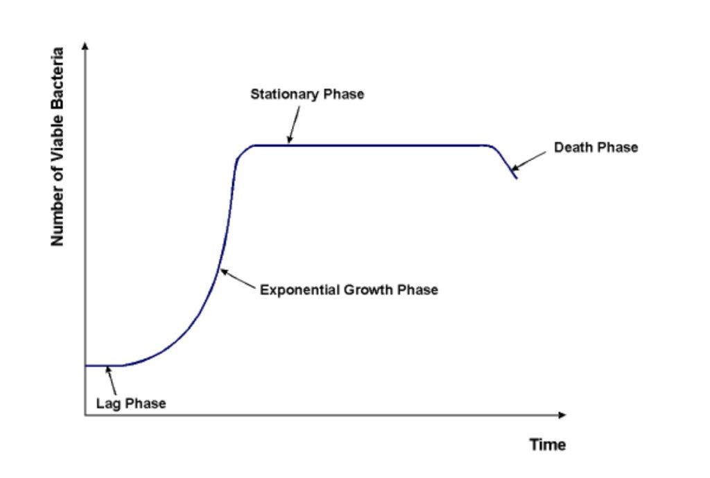
1. Lag Phase
2. Exponential Phase
3. Stationary Phase
4. Death Phase

The lapse of these phases provides data that can be compiled into a bacterial growth curve. During the lag phase, freshly cultured bacteria adjust to the media they’ve been placed in or on. As they get a feel for their surroundings and nutritional options, the cells increase enzyme production and cell size accordingly. The cells have entered the exponential phase when they begin to grow and divide at a constant pace. This phase is also called the logarithmic phase because growth occurs very rapidly and the cell count can reach into the millions and billions. As such, the number of cells is calculated using logarithmic functions. Metabolic processes also occur at a constant rate and are influenced by conditions such as pH, temperature, and properties of the medium. The stationary phase is marked by a plateau in growth. Cell death and proliferation are roughly equal. Nutrients are increasingly depleted, toxins accumulate, and cell viability decreases. The death phase occurs when these conditions cause a greater rate of cell mortality than cell proliferation. The population begins to decline at a once again exponential rate. 

Bacterial growth curves are important for calculating generation time. Generation time is the time it takes for two new cells to arise from an original cell. If starting with an inoculum with a known number of bacteria, periodic sampling can be done to calculate the generation time using the equation:

• GT is generation time
• t is the time interval between measurements b and B
• B is the initial population
• b is the population after time t

 The two most common classroom methods to determine bacterial growth are the Standard Plate Count (SPC) technique and turbidimetric measurement. Examples of other methods include: microscopic count, membrane filter count, nitrogen determination, cellular weight determination, and biochemical activity measurement. 

 Plotting a Bacterial Growth Using Turbidimetric Determination

Turbidimetric determination is useful for plotting growth curves of bacteria in broth or liquid media. It is one of the simplest methods used to analyze trends in growth because it uses a spectrophotometer to track changes in the optical density (OD) over time. In other words: as the number of cells in a sample increase, the transmission of light through the sample will decrease.  The standard OD setting is 660 nanometers for yellow to brown broth samples, but can be adjusted if the color is not in this range or if growth is expected to be lower or greater than average. The following is an example of a standard procedure using this method. It utilizes spectrophotometric measurements every 15 minutes for up to three hours. Be sure to keep track of time and record data appropriately.

1. Prepare sterile broth or media that will be used for inoculation. When ready to use, make sure the temperature is not too hot. The media container should be comfortable to the touch.
2. Power on a spectrophotometer and allow it to warm up, preferably for several minutes before use.
3. Set the wavelength of the spectrophotometer to 660 nm (or another appropriate setting). Add 5 mL of uninoculated sterile media to a clean cuvette and blank the machine by setting it to 0 ABS with this sample. This step standardizes the turbidity of the media without any cells in it, so that further calculations can quantitate growth due to changes in the turbidity.
4. Incolulate the primary media from which samples will be taken.
5. Immediately after inoculating, take a 5 mL sample of the inoculated media and pipette it into a clean cuvette. Place it in the blanked spectrophotometer, and record the OD reading. This reading should be recorded at time “0”.
6. Repeat the previous step at 15 minute intervals until the absorbance no longer increases.
7. Plot the readings on a graph with Time as the X-axis and OD as the Y-axis.

 Turbidimetric determination is very helpful for plotting a standard growth curve; it allows us to easily track changes in growth phases without the hassle of counting plated colonies. It is simple and easy; however, other procedures often provide more detailed, quantitative information and are preferred when more precise data is necessary. Turbidimetric methods can often be used alongside these other techniques as a reinforcement to trends in the data collected. Whether it is used alone or alongside other techniques, it is a simple and efficient approach when collecting data for standard growth curves.